Example Codes and Miniapps

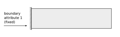
Example 1: Laplace Problem

This example code demonstrates the use of MFEM to define a simple isoparametric finite element discretization of the Laplace problem

$$-\Delta u = 1$$ with homogeneous Dirichlet boundary conditions. Specifically, we discretize with the finite element space coming from the mesh (linear by default, quadratic for quadratic curvilinear mesh, NURBS for NURBS mesh, etc.)

The example highlights the use of mesh refinement, finite element grid functions, as well as linear and bilinear forms corresponding to the left-hand side and right-hand side of the discrete linear system. We also cover the explicit elimination of essential boundary conditions, static condensation, and the optional connection to the GLVis tool for visualization.

The example has a serial (ex1.cpp), a parallel (ex1p.cpp), and HPC versions: performance/ex1.cpp, performance/ex1p.cpp. It also has a PETSc modification in examples/petsc.

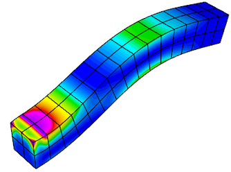
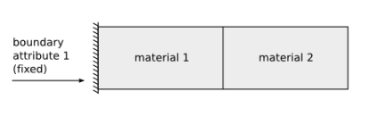
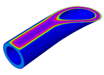
Example 2: Linear Elasticity

This example code solves a simple linear elasticity problem describing a multi-material cantilever beam. Specifically, we approximate the weak form of

$$-{\rm div}({\sigma}({\bf u})) = 0$$ where $${\sigma}({\bf u}) = \lambda\, {\rm div}({\bf u})\,I + \mu\,(\nabla{\bf u} + \nabla{\bf u}^T)$$ is the stress tensor corresponding to displacement field ${\bf u}$, and $\lambda$ and $\mu$ are the material Lame constants. The boundary conditions are ${\bf u}=0$ on the fixed part of the boundary with attribute 1, and ${\sigma}({\bf u})\cdot n = f$ on the remainder with $f$ being a constant pull down vector on boundary elements with attribute 2, and zero otherwise. The geometry of the domain is assumed to be as follows:

The example demonstrates the use of high-order and NURBS vector finite element spaces with the linear elasticity bilinear form, meshes with curved elements, and the definition of piece-wise constant and vector coefficient objects. Static condensation is also illustrated.

The example has a serial (ex2.cpp) and a parallel (ex2p.cpp) version. It also has a PETSc modification in examples/petsc. We recommend viewing Example 1 before viewing this example.

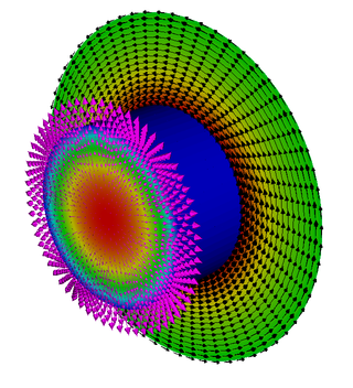
Example 3: Definite Maxwell Problem

This example code solves a simple 3D electromagnetic diffusion problem corresponding to the second order definite Maxwell equation

$$\nabla\times\nabla\times\, E + E = f$$ with boundary condition $E \times n$ = "given tangential field". Here, we use a given exact solution $E$ and compute the corresponding r.h.s. $f$. We discretize with Nedelec finite elements in 2D or 3D.

The example demonstrates the use of $H(curl)$ finite element spaces with the curl-curl and the (vector finite element) mass bilinear form, as well as the computation of discretization error when the exact solution is known. Static condensation is also illustrated.

The example has a serial (ex3.cpp) and a parallel (ex3p.cpp) version. It also has a PETSc modification in examples/petsc. We recommend viewing examples 1-2 before viewing this example.

Example 4: Grad-div Problem

This example code solves a simple 2D/3D $H(div)$ diffusion problem corresponding to the second order definite equation

$$-{\rm grad}(\alpha\,{\rm div}(F)) + \beta F = f$$ with boundary condition $F \cdot n$ = "given normal field". Here we use a given exact solution $F$ and compute the corresponding right hand side $f$. We discretize with the Raviart-Thomas finite elements.

The example demonstrates the use of $H(div)$ finite element spaces with the grad-div and $H(div)$ vector finite element mass bilinear form, as well as the computation of discretization error when the exact solution is known. Bilinear form hybridization and static condensation are also illustrated.

The example has a serial (ex4.cpp) and a parallel (ex4p.cpp) version. It also has a PETSc modification in examples/petsc. We recommend viewing examples 1-3 before viewing this example.

Example 5: Darcy Problem

This example code solves a simple 2D/3D mixed Darcy problem corresponding to the saddle point system

$$\begin{array}{rcl} k\,{\bf u} + {\rm grad}\,p &=& f \\ -{\rm div}\,{\bf u} &=& g \end{array}$$ with natural boundary condition $-p =$ "given pressure". Here we use a given exact solution $({\bf u},p)$ and compute the corresponding right hand side $(f, g)$. We discretize with Raviart-Thomas finite elements (velocity $\bf u$) and piecewise discontinuous polynomials (pressure $p$).

The example demonstrates the use of the BlockMatrix and BlockOperator classes, as well as the collective saving of several grid functions in a VisIt visualization format.

The example has a serial (ex5.cpp) and a parallel (ex5p.cpp) version. It also has a PETSc modification in examples/petsc. We recommend viewing examples 1-4 before viewing this example.

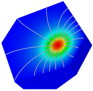
Example 6: Laplace Problem with AMR

This is a version of Example 1 with a simple adaptive mesh refinement loop. The problem being solved is again the Laplace equation

$$-\Delta u = 1$$ with homogeneous Dirichlet boundary conditions. The problem is solved on a sequence of meshes which are locally refined in a conforming (triangles, tetrahedrons) or non-conforming (quadrilateral, hexahedrons) manner according to a simple ZZ error estimator.

The example demonstrates MFEM's capability to work with both conforming and nonconforming refinements, in 2D and 3D, on linear, curved and surface meshes. Interpolation of functions from coarse to fine meshes, as well as persistent GLVis visualization are also illustrated.

The example has a serial (ex6.cpp) and a parallel (ex6p.cpp) version. It also has a PETSc modification in examples/petsc. We recommend viewing Example 1 before viewing this example.

Example 7: Surface Meshes

This example code demonstrates the use of MFEM to define a triangulation of a unit sphere and a simple isoparametric finite element discretization of the Laplace problem with mass term,

$$-\Delta u + u = f.$$

The example highlights mesh generation, the use of mesh refinement, high-order meshes and finite elements, as well as surface-based linear and bilinear forms corresponding to the left-hand side and right-hand side of the discrete linear system. Simple local mesh refinement is also demonstrated.

The example has a serial (ex7.cpp) and a parallel (ex7p.cpp) version. We recommend viewing Example 1 before viewing this example.

Example 8: DPG for the Laplace Problem

This example code demonstrates the use of the Discontinuous Petrov-Galerkin (DPG) method in its primal 2x2 block form as a simple finite element discretization of the Laplace problem

$$-\Delta u = f$$ with homogeneous Dirichlet boundary conditions. We use high-order continuous trial space, a high-order interfacial (trace) space, and a high-order discontinuous test space defining a local dual ($H^{-1}$) norm. We use the primal form of DPG, see "A primal DPG method without a first-order reformulation", Demkowicz and Gopalakrishnan, CAM 2013.

The example highlights the use of interfacial (trace) finite elements and spaces, trace face integrators and the definition of block operators and preconditioners.

The example has a serial (ex8.cpp) and a parallel (ex8p.cpp) version. We recommend viewing examples 1-5 before viewing this example.

Example 9: DG Advection

This example code solves the time-dependent advection equation

$$\frac{\partial u}{\partial t} + v \cdot \nabla u = 0,$$ where $v$ is a given fluid velocity, and $u_0(x)=u(0,x)$ is a given initial condition.

The example demonstrates the use of Discontinuous Galerkin (DG) bilinear forms in MFEM (face integrators), the use of explicit ODE time integrators, the definition of periodic boundary conditions through periodic meshes, as well as the use of GLVis for persistent visualization of a time-evolving solution. The saving of time-dependent data files for external visualization with VisIt is also illustrated.

The example has a serial (ex9.cpp) and a parallel (ex9p.cpp) version. It also has a SUNDIALS modification in examples/sundials and a PETSc modification in examples/petsc.

Example 10: Nonlinear Elasticity

This example solves a time dependent nonlinear elasticity problem of the form

$$\frac{dv}{dt} = H(x) + S v\,,\qquad \frac{dx}{dt} = v\,,$$ where $H$ is a hyperelastic model and $S$ is a viscosity operator of Laplacian type. The geometry of the domain is assumed to be as follows:

The example demonstrates the use of nonlinear operators, as well as their implicit time integration using a Newton method for solving an associated reduced backward-Euler type nonlinear equation. Each Newton step requires the inversion of a Jacobian matrix, which is done through a (preconditioned) inner solver.

The example has a serial (ex10.cpp) and a parallel (ex10p.cpp) version. It also has a SUNDIALS modification in examples/sundials and a PETSc modification in examples/petsc. We recommend viewing examples 2 and 9 before viewing this example.

Example 11: Laplace Eigenproblem

This example code demonstrates the use of MFEM to solve the eigenvalue problem

$$-\Delta u = \lambda u$$ with homogeneous Dirichlet boundary conditions.

We compute a number of the lowest eigenmodes by discretizing the Laplacian and Mass operators using a finite element space of the specified order, or an isoparametric/isogeometric space if order < 1 (quadratic for quadratic curvilinear mesh, NURBS for NURBS mesh, etc.)

The example highlights the use of the LOBPCG eigenvalue solver together with the BoomerAMG preconditioner in HYPRE, as well as optionally the SuperLU parallel direct solver. Reusing a single GLVis visualization window for multiple eigenfunctions is also illustrated.

The example has only a parallel (ex11p.cpp) version. We recommend viewing Example 1 before viewing this example.

Example 12: Linear Elasticity Eigenproblem

This example code solves the linear elasticity eigenvalue problem for a multi-material cantilever beam. Specifically, we compute a number of the lowest eigenmodes by approximating the weak form of

$$-{\rm div}({\sigma}({\bf u})) = \lambda {\bf u} \,,$$ where $${\sigma}({\bf u}) = \lambda\, {\rm div}({\bf u})\,I + \mu\,(\nabla{\bf u} + \nabla{\bf u}^T)$$ is the stress tensor corresponding to displacement field $\bf u$, and $\lambda$ and $\mu$ are the material Lame constants. The boundary conditions are ${\bf u}=0$ on the fixed part of the boundary with attribute 1, and ${\sigma}({\bf u})\cdot n = f$ on the remainder. The geometry of the domain is assumed to be as follows:

The example highlights the use of the LOBPCG eigenvalue solver together with the BoomerAMG preconditioner in HYPRE. Reusing a single GLVis visualization window for multiple eigenfunctions is also illustrated.

The example has only a parallel (ex12p.cpp) version. We recommend viewing examples 2 and 11 before viewing this example.

Example 13: Maxwell Eigenproblem

This example code solves the Maxwell (electromagnetic) eigenvalue problem

$$\nabla\times\nabla\times\, E = \lambda\, E$$ with homogeneous Dirichlet boundary conditions $E \times n = 0$.

We compute a number of the lowest nonzero eigenmodes by discretizing the curl curl operator using a Nedelec finite element space of the specified order in 2D or 3D.

The example highlights the use of the AME subspace eigenvalue solver from HYPRE, which uses LOBPCG and AMS internally. Reusing a single GLVis visualization window for multiple eigenfunctions is also illustrated.

The example has only a parallel (ex13p.cpp) version. We recommend viewing examples 3 and 11 before viewing this example.

Example 14: DG Diffusion

This example code demonstrates the use of MFEM to define a discontinuous Galerkin (DG) finite element discretization of the Laplace problem

$$-\Delta u = 1$$ with homogeneous Dirichlet boundary conditions. Finite element spaces of any order, including zero on regular grids, are supported. The example highlights the use of discontinuous spaces and DG-specific face integrators.

The example has a serial (ex14.cpp) and a parallel (ex14p.cpp) version. We recommend viewing examples 1 and 9 before viewing this example.

Example 15: Dynamic AMR

Building on Example 6, this example demonstrates dynamic adaptive mesh refinement. The mesh is adapted to a time-dependent solution by refinement as well as by derefinement. For simplicity, the solution is prescribed and no time integration is done. However, the error estimation and refinement/derefinement decisions are realistic.

At each outer iteration the right hand side function is changed to mimic a time dependent problem. Within each inner iteration the problem is solved on a sequence of meshes which are locally refined according to a simple ZZ error estimator. At the end of the inner iteration the error estimates are also used to identify any elements which may be over-refined and a single derefinement step is performed. After each refinement or derefinement step a rebalance operation is performed to keep the mesh evenly distributed among the available processors.

The example demonstrates MFEM's capability to refine, derefine and load balance nonconforming meshes, in 2D and 3D, and on linear, curved and surface meshes. Interpolation of functions between coarse and fine meshes, persistent GLVis visualization, and saving of time-dependent fields for external visualization with VisIt are also illustrated.

The example has a serial (ex15.cpp) and a parallel (ex15p.cpp) version. We recommend viewing examples 1, 6 and 9 before viewing this example.

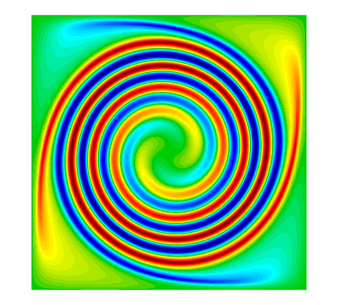
Example 16: Time Dependent Heat Conduction

This example code solves a simple 2D/3D time dependent nonlinear heat conduction problem

$$\frac{du}{dt} = \nabla \cdot \left( \kappa + \alpha u \right) \nabla u$$ with a natural insulating boundary condition $\frac{du}{dn} = 0$. We linearize the problem by using the temperature field $u$ from the previous time step to compute the conductivity coefficient.

This example demonstrates both implicit and explicit time integration as well as a single Picard step method for linearization. The saving of time dependent data files for external visualization with VisIt is also illustrated.

The example has a serial (ex16.cpp) and a parallel (ex16p.cpp) version. We recommend viewing examples 2, 9, and 10 before viewing this example.

Example 17: DG Linear Elasticity

This example code solves a simple linear elasticity problem describing a multi-material cantilever beam using symmetric or non-symmetric discontinuous Galerkin (DG) formulation.

Specifically, we approximate the weak form of

$$-{\rm div}({\sigma}({\bf u})) = 0$$ where $${\sigma}({\bf u}) = \lambda\, {\rm div}({\bf u})\,I + \mu\,(\nabla{\bf u} + \nabla{\bf u}^T)$$ is the stress tensor corresponding to displacement field ${\bf u}$, and $\lambda$ and $\mu$ are the material Lame constants. The boundary conditions are Dirichlet, $\bf{u}=\bf{u_D}$, on the fixed part of the boundary, namely boundary attributes 1 and 2; on the rest of the boundary we use ${\sigma}({\bf u})\cdot n = {\bf 0}$. The geometry of the domain is assumed to be as follows:

The example demonstrates the use of high-order DG vector finite element spaces with the linear DG elasticity bilinear form, meshes with curved elements, and the definition of piece-wise constant and function vector-coefficient objects. The use of non-homogeneous Dirichlet b.c. imposed weakly, is also illustrated.

The example has a serial (ex17.cpp) and a parallel (ex17p.cpp) version. We recommend viewing examples 2 and 14 before viewing this example.

Volta Miniapp: Electrostatics

This miniapp demonstrates the use of MFEM to solve realistic problems in the field of linear electrostatics. Its features include:

• dielectric materials
• charge densities
• surface charge densities
• prescribed voltages
• applied polarizations
• high order meshes
• high order basis functions
• adaptive mesh refinement
• advanced visualization

For more details, please see the documentation in the miniapps/electromagnetics directory.

The miniapp has only a parallel (volta.cpp) version. We recommend that new users start with the example codes before moving to the miniapps.

Tesla Miniapp: Magnetostatics

This miniapp showcases many of MFEM's features while solving a variety of realistic magnetostatics problems. Its features include:

• diamagnetic and/or paramagnetic materials
• ferromagnetic materials
• volumetric current densities
• surface current densities
• external fields
• high order meshes
• high order basis functions
• adaptive mesh refinement
• advanced visualization

For more details, please see the documentation in the miniapps/electromagnetics directory.

The miniapp has only a parallel (tesla.cpp) version. We recommend that new users start with the example codes before moving to the miniapps.

Joule Miniapp: Transient Magnetics and Joule Heating

This miniapp solves the equations of transient low-frequency (aka eddy current) electromagnetics, and simultanesously computes transient heat transfer with the heat source given by the electromagnetic Joule heating.

Its features include:

• $H^1$ discretization of the electrostatic potential
• $H(\mathrm{curl})$ discretization of the electric field
• $H(\mathrm{div})$ discretization of the magetic field
• $H(\mathrm{div})$ discretization of the heat flux
• $L^2$ discretization of the temperature
• implicit transient time integration
• high order meshes
• high order basis functions
• adaptive mesh refinement
• advanced visualization

For more details, please see the documentation in the miniapps/electromagnetics directory.

The miniapp has only a parallel (joule.cpp) version. We recommend that new users start with the example codes before moving to the miniapps.

Mobius Strip Miniapp

This miniapp generates various Mobius strip-like surface meshes. It is a good way to generate complex surface meshes.

Manipulating the mesh topology and performing mesh transformation are demonstrated.

The mobius-strip mesh in the data directory was generated with this miniapp.

For more details, please see the documentation in the miniapps/meshing directory.

The miniapp has only a serial (mobius-strip.cpp) version. We recommend that new users start with the example codes before moving to the miniapps.

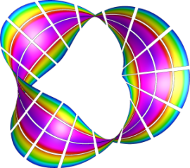
Klein Bottle Miniapp

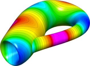
This miniapp generates three types of Klein bottle surfaces. It is similar to the mobius-strip miniapp.

Manipulating the mesh topology and performing mesh transformation are demonstrated.

The klein-bottle and klein-donut meshes in the data directory was generated with this miniapp.

For more details, please see the documentation in the miniapps/meshing directory.

The miniapp has only a serial (klein-bottle.cpp) version. We recommend that new users start with the example codes before moving to the miniapps.

Mesh Explorer Miniapp

This miniapp is a handy tool to examine, visualize and manipulate a given mesh. Some of its features are:

• visualizing of mesh materials and individual mesh elements
• mesh scaling, randomization, and general transformation
• manipulation of the mesh curvature
• the ability to simulate parallel partitioning
• quantitative and visual reports of mesh quality

For more details, please see the documentation in the miniapps/meshing directory.

The miniapp has only a serial (mesh-explorer.cpp) version. We recommend that new users start with the example codes before moving to the miniapps.

No examples or miniapps match your criteria.

---